|
|
Loading...
Searching...
No Matches
|
|
Primarily, Rack computes meteorological products in polar coordinate system. The resulting product is also in polar coordinates, hence called a polar product. It can be also called as an intermediate product because such a product is often processed further on, for example added to a composite or transformed to a Cartesian single-radar image. This design feature adds speed to production since many final products can be computed from the same polar product. This also facilitates developing the software, as a new meteorological algorithm needs to be programmed in a single module only.
By default, generation of a product removes the previous product from memory. Alternatively, several products can be written in the same output structure by issuing --append dataset or --append data (with optional index) before the product commands..
The rest of this section handles computation of polar products. Since end products are most often viewed in Cartesian coordinates and coloured, the examples include the Cartesian conversion (-c) and palette operation (--palette ). A quality field, when provided by the product operator, is attached right of the actual product image.
As processing and using Doppler data involves special aspects, it is handled in it own section, Basic Doppler products.
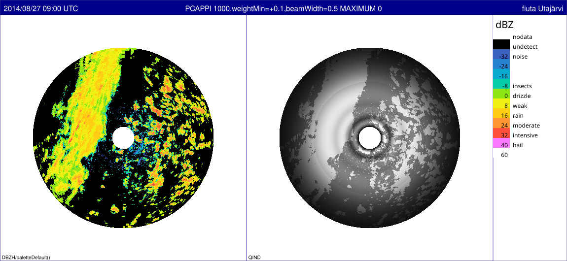
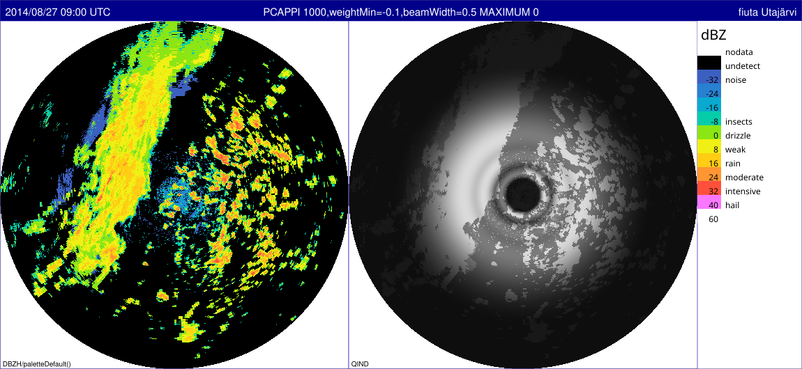
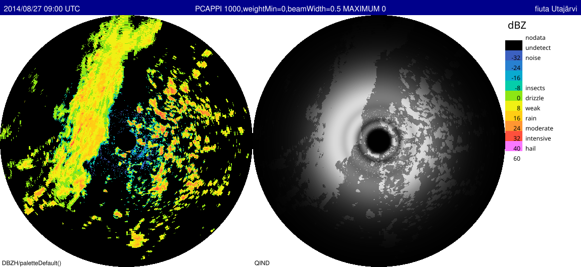
Constant-altitude position indicator (CAPPI) is obtained with --pCappi command. It takes altitude as its first argument.
The Pseudo CAPPI product is computed by traversing all the bins of the volume data. The bins are weighted using an exponential function of the distance from reference altitude. This method allows using measurement data from upper and lower beams, when data has low quality or data is missing in the closest bins.
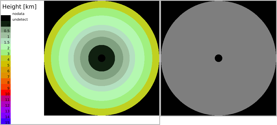
Rack supports computing three variations of CAPPI. They differ in ways vertically distant data – bins far below and above the requested altitude – near and far from the radar hence are handled.
weightMin > 0, dropping low-quality areas ie. marking them with nodata , resulting in an annular shaped image weightMin < 0, including data far off the nominal altitudeweightMin = 0, dropping low-quality areas ie. marking them with undetect , resulting in an annular shaped image The images below illustrate these variations. Virtual beam width has been set smaller (0.5) to visualize the differences and the quality field.
As a default setting, the relative quality of undetect bins is lower than that of detected signals; this affects e.g. creation of radar image composites. The relative quality can be changed with --undetectWeight command.
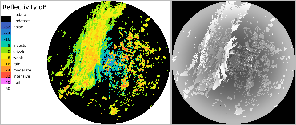
Maximum reflectivity in vertical direction is obtained --maxEcho command. It takes two parametes: (minimum) altitude above which reflectances are considered and altitudeDev (altitude deviation), a fuzzy width parameter of the threshold.
The quality is low near and far from the radar, as precipitation may reside over and under radar beams, respectively.
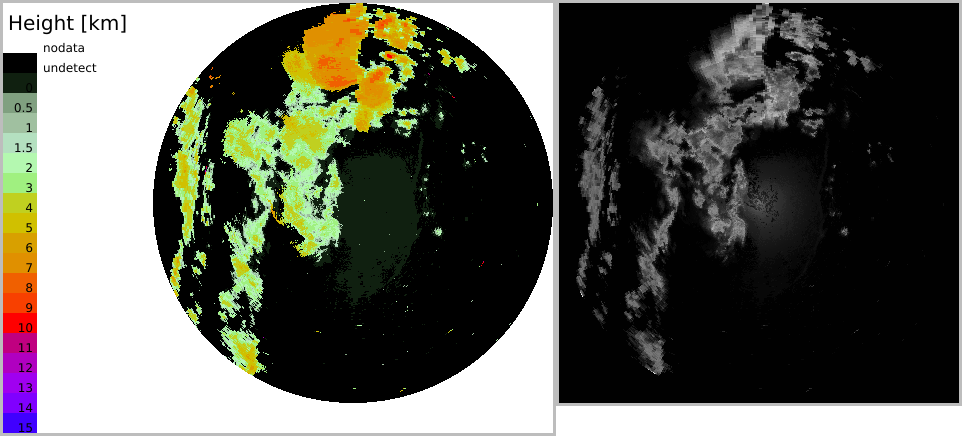
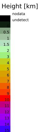
Height of precipitation can be computed with --pEchoTop command. It takes threshold reflectivity (dBZ) as its first argument.
The other parameters are the coordinates of a hight reference point having a very low dBZ value. The echo top altitudes are linearly interpolated towards this point.
The user may wish to choose a target resolution, for example:
Class probability for convective precipitation is obtained with --pConv command.
(Under constr.)
Currently, rack provides two operators for estimating instantaneous rainfall rate: an operator using single and another using double polarization. The rate is estimated aloft, ie. on an elevation scan (by default the lowest one). That is, there is currently no actual surface rainfall rate estimation. The computation uses the following formulae:


The parameters of these formulae can be changed with the respective commands:
These commands can be seen collectively also with --help formulae .
The simpler command --pRainRate uses --precipZrain and --precipZsnow . It assumes that a global freezing level is available in data as ODIM variable how:freeze [km]. To override that, the user may apply --freezingLevel to set the height and thickness of the freezing level.
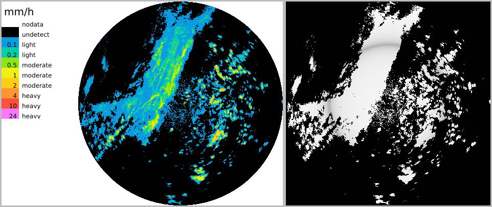
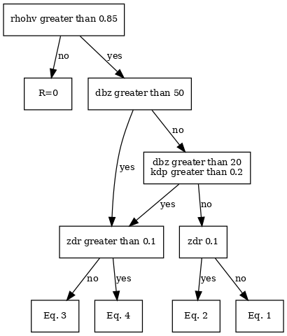
Calculates the rain rate using four different functions that utilize dbz, zdr and kdp data. The optimal rain rate function is chosen for each radar data pixel using the given data threshold values. These thresholds are adjustable and their values can be given from the command line, for example:
where the values are:
The functions are:
(1) 
(2) 
(3) 
(4) 
The graph describes the rain rate calculation algorithm that mixes all the four methods. Dual pol. equations shouldn't be applied if the measurement is done closer than 10 km from the radar. In addition, the equations should only be used for liquid water. These factors have been taken into consideration in the implementation and Eq.1 is used when ever the other equations can't be applied.
Vertical distribution of reflectivity can be computed with --verticalProfile . It takes several arguments:
The default selector for this operator defines quantity=^DBZH$ but more quantities can included with --select . The resulting product consists of one-dimensional arrays for height (HGHT ) and each input quantity stored in data groups, /dataset1/data <N> . In addition to the native output format (HDF5), the resulting product can exported as an image (png) or text (mat format). The latter works only if azSlots=1 , for example:
The text file consists of a header line and the quantities in column layout. Height (HGHT) will be always the first quantity:
The text format suits well to further illustrations with appropriate software. The curve images below have been created with gnuplot .

Both the applied input quantities and the output quantities can be set with --select command.
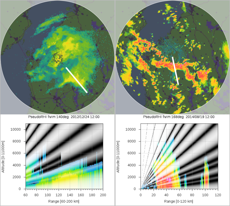
While a true Range-height indicator (RHI) is obtained by tilting the radar antenna vertically, one may construct Pseudo RHI's by computing an intersection in a standard measurement volume consisting of azimuthal sweeps.
Such a product is obtained with
Experimental. Using Rack Python API, the respective product can be created with:
The 2D data may be coloured with --palette command and saved as an image file. The gridded images below have been created from such images with gnuplot .
For special applications, the height of the beam can be computed with --beamAltitude command. It takes the altitude reference point as argument (0=radar site, 1=sea level), Target properties can be set with --encoding command: image type (typically 'C' or 'd') as the first argument and gain (kilometres) as second. The resulting polar product is simply a function of ground distance, hence an array of nbins x 1 elements, but can be projected to a Cartesian product like any other polar product.
 1.9.8
1.9.8