|
|
Loading...
Searching...
No Matches
|
|
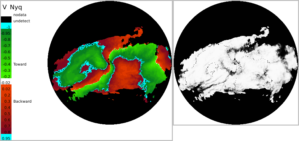
In radar meteorologically, motion can be divided to two phenomenon: atmospheric motion, which is motion of air and falling hydrometeors, and motion of precipitation area, which can be further divided into motion of convective and stratiform areas, for example. Rack is capable of detecting both of them.
Weather radars capable of measuring Doppler speed produce hydrometeor velocities projected on the beam – hence one-dimensional. The obtained speeds are further aliased by the maximum unambiguous velocity, 
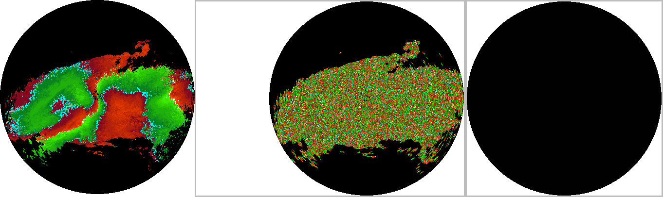
The Doppler field can be smoothed with --pDopplerAvg command:
There are several parameters, determining the window width and height, minimum percentage for the samples in the window, switch for compensating the beam broadening, as well as switch for scaling the result with maximum unambiguous speed 
how:NI in ODIM metadata).
There is also an exponential (yet asymmetric) --pDopplerAvgExp . It is recommended to use at least 16-bit resolution to store averaged fields.
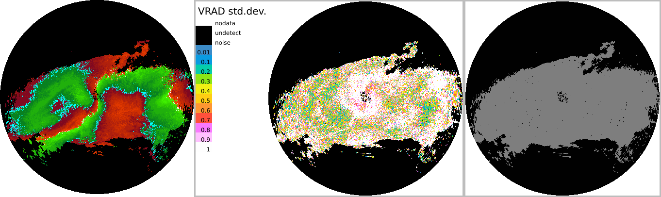
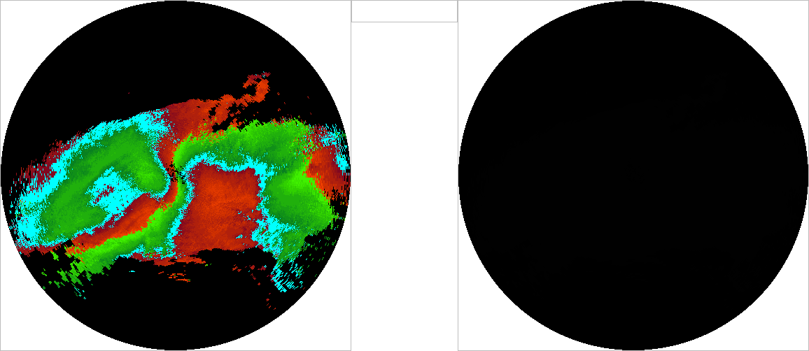
The standard deviation in Doppler field can be displayed with --pDopplerDev command.
The parameters are the same as in the Doppler averaging above.
See also the corresponding anomaly detector: Detecting variations in Doppler wind .
Basic usage creates polar products, ie. a resulting array is in polar coordinates:
The vector field can be stored in text format to as follows:
The filename has to have "dat" as extension. See Sampling data for further instructions of using --sample. The output (truncated in the middle) is as follows:
Typically, user wants to obtain a Cartesian array, obtained with --cCreate, abbreviated -c . That operation has to be performed separately for u and v components, and using --append command to prevent overwriting:
The resulting motion fields will be in the last available dataset group, here dataset1 . This behaviour can be changed with --append dataset which puts AMVU and AMVV in separate groups.
Similarly, cartesian sampling is done basically by changing extension .h5 to .dat
producing:
Accompanied utility script draw-vectors.sh creates plots of vector fields using gnuplot utility. The original data can be in text (.dat) or HDF5 (.h5) format. Optional background images can be applied. For example:
As shown above, Rack produces wind fields (u,v) directly, but also de-aliased Doppler fields can be computed. This is obtained by re-projecting the approximated (u,v) data back to radar beams and matching the result with the original aliased data. This approach cancels the smoothing effect apparent in the approximated (u,v) field. Dealiasing is done by setting nyquist parameter to a desired virtual maximum speed, say 50m/s:

Alternatively, one may skip matching of the original and derived velocities with matchAliased=0 , resulting in smoother images.

Rack provides commands for extracting atmospheric motion vectors (AMV's). There are two approaches:
Both approaches are based on least-squares fitting applying matrix inversion.
The technique is called optical flow, and is based on computing spatial and temporal differentials. Further, the implementation in Rack applies sliding window techniques which makes the approach computationally quick even with windows of size 75x75, for example.
The command, --cOpticalFlow , takes several parameters. The first two define the size of the sliding window.
The third parameter is an optional threshold, for example 0 (dBZ) in case of reflectivity data. Thresholding may be needed in order to filter apparent echo area edges caused radar geometry and sensitivity.
Smoothing (1=true) is always recommended especially with radar images that have large areas of empty data ie. "undetected" echoes. Alternatively, radar data can be smoothed by some separate process or previous commands, say --iAverage or --iGaussianAverage.
The input should contain two Cartesian datasets, for example composites. An optimal time difference between the files is typically 15 or 30 minutes. Such file can be generated for example with
The actual processing is done as follows:
The resulting file contains horizontal motion vector (u, v) stored in quantities AMVU and AMVV . In addition, a quality field (with QIND ) is provided. In addition, if --store INTERMEDIATE is set, then the following fields are stored:
Note that the above commands can be combined to a single command line, avoiding creation of intermediate file (composite-pair.h5 ).
As with Doppler motion, script draw-vectors.sh can be used for visualizing the result:

Both methods described above produce an incomplete motion field: Doppler dealiasing provides realiable vectors inside wide-spread precipitation whereas optical flow based motion analysis works best with visual details like edges and specks. Rack provides some methods for spreading the vector fields, with optional support of quality information. The methods are essentially image operators described in Image processing.
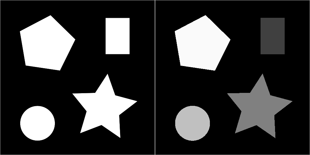
The spreading methods for two dimensional motion vectors are illustrated using an artificial image of "clouds" shown below. In vectors, high, intermediate, and low quality are illustrated in green, blue and pink colour, respectively. Utility script draw-vectors.sh and GnuPlot have been used in creating the visualisations below.
An straighforward way to spread scalar or vector data is to apply a smoothing window on data. In Rack, fast and simple smoothing is carried out using rectangular averaging window:

--iAverage, window size 200 x 200.As a computational speed-up, the rectangular averaging window of size 


Two-dimensional Gaussian bell function produces smooth fields. Also that operator can be a separated to two consecutive one-dimensional run of

--iGaussianAverage, window size 400 x 400.Sometimes it is desired that opposite vector components do not cancel each other but the magnitudes be preserved like in a flow a fluid or particles. Using --iFlowAverage produces such vectors, pointing to directions of conventionally averaged vectors.

--iFlowAverage, window size 200 x 200.The shape of this window operator is rectangular, and basically cannot be accelerated ie. separated to two operations with narrow windows. Technically, such processing can be performed by issuing the commands explicitly, producing an approximation of the true rectangular window operation:
The problem with all the averaging operators is that they also blur areas of high-quality vectors. As a solution, the vectors of low quality in the resulting image should be overridden with vectors of higher quality of the original image. This kind of combination can be produced repeatedly using --iBlender which employs a desired averaging operator (above) with a maximum or mixing operator with the original image:

--iBlender, window size 200 x 200, applying simple averaging and maximum-quality combination.An alternative way to spead vector fields is to apply distance transform based methods: data values are propagated in all the directions such that the underlying quality field is decreased as a function of distance.
Propagation continues in low-quality areas until higher quality values are encountered. This method is very fast, but as a disadvantage the resulting vector fields contain segments of constant values as no averaging is involved. The basic version is applies linear model ie. constant steps in decreasing the underlying quality field. If the data has no quality data, it can be created with --createDefaultQuality .
--iDistanceTransformFill, window size 200 x 200.When using distance transform approach, an area of high quality may override an area of lower quality if the areas are close enough like in the upper right corner of the sample image (the motion field of the pentagon overrides that of the rectangle). When using an exponential model, the resulting quality field has steeply decaying values - that however continue to infinity, in the limits of storage type precision.
--iDistanceTransformFillExp, window size 200 x 200.The linear and exponential approaches have same the computional complexity.
It is possible to generate composites of single-radar motion fields presented above. The procedure is essenstially the same as with intensity data, explained in Cartesian conversions and composites . However, compositing has to be done separately for each parameter, in this case horizontal wind components AMVU and AMVV .
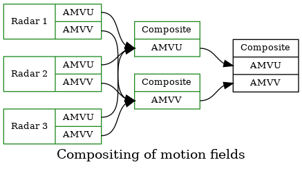
For example, assuming that –c <files> are a set of motion files to be composites:
Note that the input files can be the same in the above lines, if they contain both the quantities.
 1.9.8
1.9.8