Point data

Table of Contents

• Adding point measurements
  • Rain rate observations
  • Aviation obstacles

Adding point measurements

Also external point measurements - like ground station observations - can be projected into a Cartesian product. Technically, the procedure works as in compositing, which applies internally an accumulation array: adding data from a single radar is equal to adding several single observations.

Everything starts by creating an empty accumulation array with –cSize and –cProj commands; sometimes –cMethod may apply as well. Alternatively, the array can be initialised with a radar composite by loading it with –cLoad . Moreover, plotting can be arbitrarily mixed with single radar observations; weighting can be applied in tuning the between radars and ground observations.

Single entries can be added in a command line with –cPlot command. The command has the form

rack <composite-settings> --cPlot <lon>,<lat>,<intensity>[,<weight>] [...] --cExtract dw  [--cSpread <spread>]  <output-commands> 

The plotting command takes longitude, latitude and intensity as parameters. Intensity is the magnitude of the user defined quantity, say rain rate. A weight parameter can be associated to each observation. After extraction, the pointwise intensities can be spread coarsely as ellipses using –cSpread , which takes horizonal and vertical radii in kilometres as arguments. Like any other products, the result can be stored in an HDF5 or image file.

Rain rate observations

Applying many subsequent –cPlot commands is clumsy.
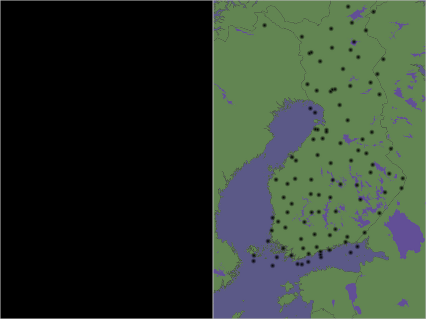
Assume that you have file measurements.dat containing comma separated entries of lon,lat, and measurement value, like

# lon,lat,mmh
  20.78302  69.03332         0
  20.78302  69.03332         0
  23.96628  66.76636         0
  23.96628  66.76636         0
  24.71638  64.03332        .6
...
    ...
        ...
  26.96628  65.38318         0
  26.96628  65.38318         0
   29.1666  67.14994         0
   25.0833  64.68306         0
  29.31654  66.36652         0

then you can plot them with –cPlotFile command as follows:

#!/bin/bash
 
INFILE=${INFILE:-$1}
INFILE=${INFILE:-'measurements.dat'}
QUANTITY=${QUANTITY:-'RATE'}
GAIN=${GAIN:-'0.02'}
ENCODING=${ENCODING:-"C,gain=${GAIN},offset=-${GAIN},undetect=254,nodata=0,quantity=${QUANTITY}"}
# Finland
BBOX=${BBOX:-'17,57.75,32.75,70'}
SIZE=${SIZE:-'500,750'}
 
#palette=`ls palette-${QUANTITY}.{json,txt}` &> /dev/null
cmd="rack  --cProj '+proj=longlat +ellps=WGS84 +datum=WGS84 +no_defs' --cBBox $BBOX  --cSize $SIZE  \
  --encoding ${ENCODING} \
  --cPlotFile ${INFILE} \
  --cExtract dw \
  -o plot.png \
  --iDistanceTransformFill 7 \
  -o plot-spread1.png  \
  --palette '$QUANTITY' --paletteRefine 64  -o plot-spread-color.png  "
 
#   --palette $palette --paletteRefine 64  -o plot-spread-color.png  "
 
 
#  --palette palette-RATE.txt --paletteRefine 64 --imageTransp 0,0.5,0.2  -o plot-spread-color.png  
#  --palette palette-RATE.txt --paletteRefine 64 --imageTransp 0:2,0.5,0.2 -o plot-spread-color.png  
#   --encoding C,gain=${GAIN},offset=-${GAIN},undetect=254,nodata=0,quantity=${QUANTITY} \
 
echo $cmd
eval $cmd
 
#  -o plot-spread2.h5  \
#  --iGaussianAverage 15 \
#  -o plot-spread2.png  \
#  --iGaussianAverage 15 \
#  --iAverage 15 \
 
 

For further processing, it may be needed to add several ODIM variables as in the above script.

Rainfall observations plotted and spread to 50km circles (left) and similar 100km circles coloured with --palette and superposed on a map (right).

Aviation obstacles